Introduction to Deep Convolutional Neural Networks

Deep Convolutional Neural Networks (DCNNs) are a specialized type of neural network architecture that excels in analyzing visual data. They are a subclass of Convolutional Neural Networks (CNNs) designed with many layers, which allows them to automatically learn hierarchical feature representations from raw input images. DCNNs have proven to be highly effective in various tasks such as image classification, object detection, segmentation, and even in fields like medical imaging and natural language processing. Their ability to extract spatial features at multiple levels has made them a dominant model in computer vision tasks.

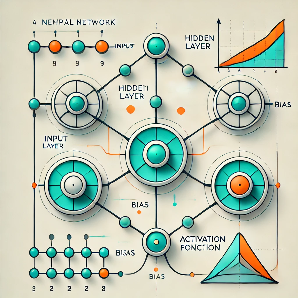
Basic Structure of DCNNs

• Input Layer: The input layer takes in raw pixel values of an image, typically in the form of a multi-dimensional matrix (height x width x channels).
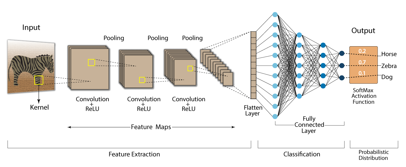
• Convolutional Layers: These layers perform convolution operations to extract local features from the input data. Each convolution operation involves sliding a filter (kernel) over the image to capture spatial patterns such as edges, textures, and shapes.
• Activation Function: Typically, Rectified Linear Unit (ReLU) is applied after convolution to introduce non-linearity, helping the network learn more complex patterns.
• Pooling Layers: Pooling layers are used to reduce the spatial dimensions of the feature maps, typically through max pooling or average pooling, while retaining essential information.
• Fully Connected Layers: These layers are present towards the end of the network and connect every neuron to all neurons in the previous layer. They aggregate the learned features for the final decision-making process.
• Output Layer: The output layer produces the final prediction, which could be a classification label, regression value, or any other task-specific output.

Working Mechanism of DCNNs

1. Convolutional Layer

• In the convolutional layer, a filter (also called a kernel) is applied to the input image to perform convolution.
• The filter slides over the image and produces a set of feature maps that highlight various features of the image such as edges or textures.

2. Activation Function (ReLU)

• ReLU (Rectified Linear Unit) is commonly used as an activation function to introduce non-linearity in the network. It replaces all negative values with zero while leaving positive values unchanged.
• This helps the network learn more complex patterns, enabling it to model the complexity of real-world data.

3. Pooling Layer

• After convolution, the pooling layer is applied to reduce the spatial size of the feature maps. This is done to minimize computation and prevent overfitting.
• Max pooling, where the maximum value in a set of neighboring pixels is retained, is a common method used in DCNNs.

4. Fully Connected Layer

• The fully connected layer connects all neurons in the previous layers to each neuron in the current layer. This layer is responsible for decision-making based on the learned features.
• The output of the fully connected layer is then passed to the output layer for final prediction.

5. Output Layer

• The output layer is where the network produces the final result, such as a classification label (e.g., "cat" or "dog") or a continuous value in regression tasks.

Applications of DCNNs

• Image Classification: DCNNs are widely used for classifying images into categories. For example, recognizing whether an image contains a cat or a dog.
• Object Detection: DCNNs are used to identify and localize objects within an image, making them ideal for applications like autonomous vehicles and facial recognition.
• Medical Imaging: DCNNs help in analyzing medical scans, such as detecting tumors or classifying medical conditions from X-rays, MRIs, or CT scans.
• Image Segmentation: DCNNs are used to segment an image into regions of interest, which is essential in applications like image editing or autonomous driving.
• Natural Language Processing: Although DCNNs are primarily used for image data, they are also applied in text processing tasks like sentiment analysis by treating text as a sequence of tokens.

Advantages of DCNNs

• Automatic Feature Learning: DCNNs automatically learn hierarchical features from raw input data, eliminating the need for manual feature extraction.
• Translation Invariance: Due to the use of convolution and pooling, DCNNs are invariant to small translations in the input image, meaning that they can recognize an object regardless of its position.
• Robustness: DCNNs are highly effective at generalizing across different types of input data, making them robust in real-world scenarios.
• High Performance: DCNNs consistently achieve state-of-the-art performance across a wide range of computer vision tasks.

Limitations of DCNNs

• Computationally Expensive: Training deep CNNs requires large computational resources, including powerful GPUs and substantial memory.
• Requires Large Datasets: DCNNs perform best with large labeled datasets. Their performance can degrade when the amount of data is insufficient.
• Risk of Overfitting: With complex architectures and insufficient data, DCNNs are prone to overfitting, where the model learns noise rather than useful patterns.
• Limited Interpretability: DCNNs are often considered "black boxes," meaning their decision-making process is not easily interpretable, which can be a concern in high-stakes applications like healthcare.
• Slow Inference: Although DCNNs are powerful during training, they can be slow at inference time, especially when the models are deep and the input data is large.

Sample Code Example

DCNN in Action: Classifying CIFAR-10 Images with TensorFlow

    
        # Import required libraries
        import numpy as np
        import matplotlib.pyplot as plt
        from tensorflow.keras import layers, models
        from tensorflow.keras.datasets import cifar10
        from tensorflow.keras.utils import to_categorical
        
        # Load and preprocess the CIFAR-10 dataset
        (x_train, y_train), (x_test, y_test) = cifar10.load_data()
        
        # Normalize the image data to a range of [0, 1]
        x_train, x_test = x_train / 255.0, x_test / 255.0
        
        # One-hot encode the labels
        y_train = to_categorical(y_train, 10)
        y_test = to_categorical(y_test, 10)
        
        # Build the Deep Convolutional Neural Network (DCNN) model
        model = models.Sequential()
        
        # Add convolutional layers with ReLU activations and max pooling
        model.add(layers.Conv2D(32, (3, 3), activation='relu', input_shape=(32, 32, 3)))
        model.add(layers.MaxPooling2D((2, 2)))
        
        model.add(layers.Conv2D(64, (3, 3), activation='relu'))
        model.add(layers.MaxPooling2D((2, 2)))
        
        model.add(layers.Conv2D(64, (3, 3), activation='relu'))
        
        # Flatten the output from the convolutional layers and add dense layers
        model.add(layers.Flatten())
        model.add(layers.Dense(64, activation='relu'))
        
        # Output layer with softmax activation for multi-class classification
        model.add(layers.Dense(10, activation='softmax'))
        
        # Compile the model
        model.compile(optimizer='adam',
                      loss='categorical_crossentropy',
                      metrics=['accuracy'])
        
        # Train the model and save history for visualization
        history = model.fit(x_train, y_train, epochs=10, batch_size=64, 
                            validation_data=(x_test, y_test))
        
        # Evaluate the model on the test set
        test_loss, test_acc = model.evaluate(x_test, y_test, verbose=2)
        print(f"Test accuracy: {test_acc:.4f}")
        
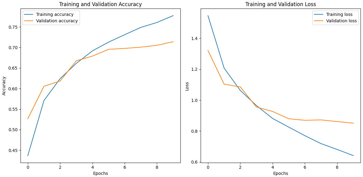
        # Visualize the training progress (accuracy and loss)
        # Plot training and validation accuracy
        plt.figure(figsize=(12, 6))
        
        # Accuracy plot
        plt.subplot(1, 2, 1)
        plt.plot(history.history['accuracy'], label='Training accuracy')
        plt.plot(history.history['val_accuracy'], label='Validation accuracy')
        plt.title('Training and Validation Accuracy')
        plt.xlabel('Epochs')
        plt.ylabel('Accuracy')
        plt.legend()
        
        # Loss plot
        plt.subplot(1, 2, 2)
        plt.plot(history.history['loss'], label='Training loss')
        plt.plot(history.history['val_loss'], label='Validation loss')
        plt.title('Training and Validation Loss')
        plt.xlabel('Epochs')
        plt.ylabel('Loss')
        plt.legend()
        
        plt.tight_layout()
        plt.show()
        


                    

                        
Output: