Introduction to Support Vector Machines

Support Vector Machines (SVM) are a class of supervised learning algorithms used for classification and regression tasks. They work by finding the hyperplane that best separates the data into different classes in a high-dimensional space.

Working Mechanism of SVM

1. Data Representation

• Feature Space:Each data point in the training set is represented as a vector in an n-dimensional feature space, where 'n' is the number of features.
• Labels: For classification, each vector (data point) is labeled according to its class, e.g., positive (+1) or negative (-1).

2.Linear Separation

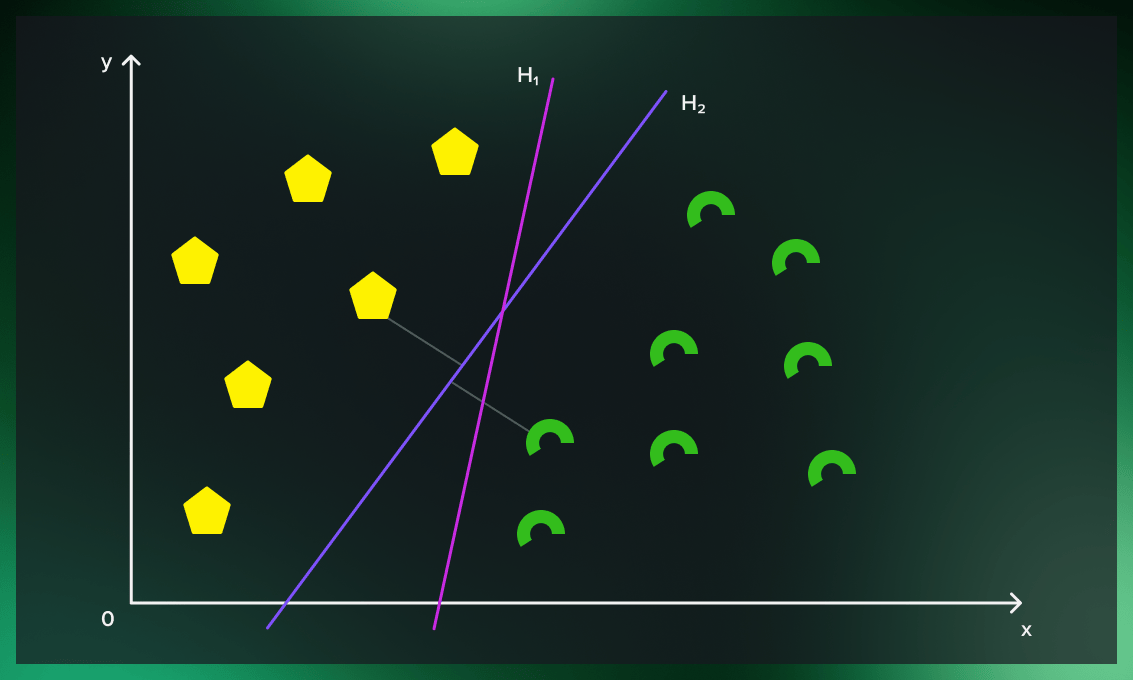
• Goal:SVM aims to find the optimal hyperplane that best separates the data points into two classes.
• Hyperplane: A hyperplane is a decision boundary that divides the feature space into two parts, with data points on either side belonging to different classes.
• Linear Separability: If the data is linearly separable, SVM identifies a straight line (in 2D) or a flat plane (in higher dimensions) that maximizes the margin between the classes.

3.Maximizing the Margin

• Margin:The margin is the distance between the hyperplane and the closest data points from each class. The goal is to maximize this margin.
• Support Vectors:Support vectors are the data points that lie closest to the hyperplane and have the most influence on its position and orientation. Only these points are used to define the optimal hyperplane.
• Optimal Hyperplane:The hyperplane is chosen such that the margin between the support vectors of different classes is maximized, reducing the risk of misclassification.

4.Handling Non-linearly Separable Data

• Kernel Trick:When data is not linearly separable, SVM uses a technique called the kernel trick. This transforms the data into a higher-dimensional space where a linear separation is possible.
• Common Kernels:
• Linear Kernel: Used when the data is linearly separable.
• Polynomial Kernel: Maps the data into higher polynomial dimensions.
• Radial Basis Function (RBF) Kernel: Useful for non-linear data, mapping it into infinite-dimensional space.
• Implicit Transformation:The kernel trick allows SVM to operate in the higher-dimensional space without explicitly computing the transformation, making it computationally efficient.

5.Soft Margin for Noisy Data

• Real-world Data: In many real-world cases, data is not perfectly separable. Outliers and noise can exist.
• Soft Margin SVM:To handle this, SVM introduces a soft margin that allows some misclassifications or violations of the margin constraints.
• Regularization Parameter (C):The regularization parameter C controls the trade-off between maximizing the margin and allowing for classification errors (soft margin). A small value of C creates a larger margin but allows more misclassifications, while a large value of C attempts to classify all points correctly but might lead to a smaller margin and potential overfitting.

6.Mathematical Formulation

• Objective:The SVM optimization problem can be formulated as:
• Maximize the margin:∣∣w∣∣
• Subject to the constraint: 𝑦 𝑖 ( 𝑤 ⋅ 𝑥 𝑖 + 𝑏 ) ≥ 1 y i ​ (w⋅x i ​ +b)≥1 for all 𝑖 i, where 𝑦 𝑖 y i ​ is the label and 𝑥 𝑖 x i ​ is the feature vector.
• Optimization Problem: This is solved using methods such as quadratic programming to find the optimal weight vector w and bias b that define the hyperplane.

7.Prediction

• Once the model is trained, the decision function for any new data point 𝑥 x is given by: 𝑓 ( 𝑥 ) = 𝑠 𝑖 𝑔 𝑛 ( 𝑤 ⋅ 𝑥 + 𝑏 ) f(x)=sign(w⋅x+b)
• The sign of this function determines the class of the data point. If 𝑓 ( 𝑥 ) f(x) is positive, the data point belongs to one class; if negative, it belongs to the other class.

8.Evaluation and Generalization

• After training the model, it is evaluated on a test set to measure performance metrics like accuracy, precision, recall, and F1-score.
• SVM aims to generalize well to unseen data by maximizing the margin and minimizing the influence of noisy data points.

Advantages of SVM

• Effective in high-dimensional spaces: SVMs work well even when the number of features is large relative to the number of samples.
• Robust to overfitting: Especially in high-dimensional settings, SVMs are effective in avoiding overfitting by focusing on support vectors.
• Flexible with different kernel functions: SVMs can use different kernels to handle non-linear data separations.

Disadvantages of SVM

• Computationally expensive: Training an SVM, especially with large datasets, can be slow and resource-intensive.
• Sensitive to choice of kernel and parameters: The performance of SVMs is highly dependent on the selection of the appropriate kernel and tuning of the parameters.
• Not well-suited for large datasets: SVMs may struggle with performance when applied to very large datasets.

Sample Code Example

Linear Regression in Action: Predicting House Prices based on Size:

        
            # svm_visualization.py

            import numpy as np
            import matplotlib.pyplot as plt
            import seaborn as sns
            from sklearn import datasets
            from sklearn.model_selection import train_test_split
            from sklearn.svm import SVC
            from sklearn.metrics import accuracy_score
            
            # Load dataset (using the Iris dataset for simplicity)
            iris = datasets.load_iris()
            X = iris.data[:, :2]  # Use only the first two features for easy 2D visualization
            y = iris.target
            
            # Train-test split
            X_train, X_test, y_train, y_test = train_test_split(X, y, test_size=0.3, random_state=42)
            
            # Create and train the SVM model
            model = SVC(kernel='linear', C=1.0)
            model.fit(X_train, y_train)
            
            # Predict the test set
            y_pred = model.predict(X_test)
            print(f"Accuracy: {accuracy_score(y_test, y_pred):.2f}")
            
            # Visualization
            def plot_decision_boundary(X, y, model):
                # Create a grid of points
                x_min, x_max = X[:, 0].min() - 1, X[:, 0].max() + 1
                y_min, y_max = X[:, 1].min() - 1, X[:, 1].max() + 1
                xx, yy = np.meshgrid(np.arange(x_min, x_max, 0.02),
                                     np.arange(y_min, y_max, 0.02))
                
                # Predict class labels for each point in the grid
                Z = model.predict(np.c_[xx.ravel(), yy.ravel()])
                Z = Z.reshape(xx.shape)
                
                # Plot the decision boundary
                plt.contourf(xx, yy, Z, alpha=0.8, cmap=sns.color_palette("coolwarm", as_cmap=True))
                
                # Plot the data points
                sns.scatterplot(x=X[:, 0], y=X[:, 1], hue=y, palette="coolwarm", edgecolor="k", s=100)
                
                # Set labels
                plt.xlabel(iris.feature_names[0])
                plt.ylabel(iris.feature_names[1])
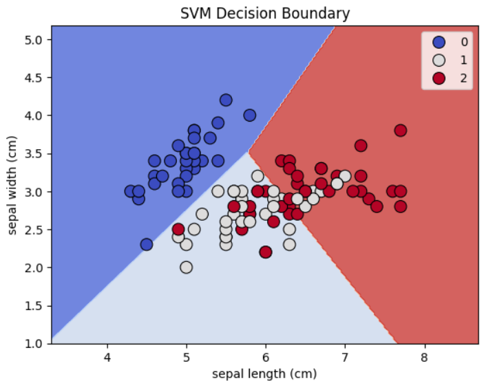
                plt.title("SVM Decision Boundary")
                plt.show()
            
            # Plot decision boundary
            plot_decision_boundary(X_train, y_train, model)
            
            
        
        
Output: