Linear Regression

Introduction to Linear Regression

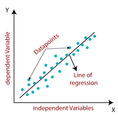
Linear regression is a statistical method used to model the relationship between a dependent variable and one or more independent variables. It assumes a linear relationship between the variables, meaning that the relationship can be represented by a straight line

The Linear Regression Equation

The equation for linear regression is:

y = mx + b

y: is the dependent variable (the one we want to predict)
x: is the independent variable (the one we use to make predictions)
m: is the slope of the line (how steep the line is)
b: is the y-intercept (where the line crosses the y-axis)

Working Mechanism of Linear Regression

1.Data Collection

Gather relevant data for the dependent and independent variables.
Ensure the data is representative of the population you want to study.

2.Data Exploration:

Visualization:Create scatter plots to visually inspect the relationship between the variables.
Correlation:Calculate the correlation coefficient to quantify the strength and direction of the linear relationship.

3.Model Building:

Define the linear regression equation:

y = mx + b

y is the dependent variable
x is the independent variable
m is the slope of the linee
b is the y-intercept

4.Parameter Estimation

Once the model is trained, it can be used to make predictions on new data:

Least Squares Method: This is the most common method to estimate the values of m and b. It minimizes the sum of the squared differences between the actual y values and the predicted y values (based on the regression line).
Normal Equations: A set of equations derived from the least squares method can be solved to find the optimal values of m and b.

5.Model Evaluation:

Goodness of Fit: Assess how well the model fits the data using metrics like:

R-squared: Measures the proportion of variance in y explained by the model.
Mean Squared Error (MSE): Measures the average squared difference between the actual and predicted values.
Root Mean Squared Error (RMSE):The square root of MSE, providing a measure in the same units as the dependent variable.

Hypothesis Testing: Use statistical tests (e.g., t-test, F-test) to determine if the model is statistically significant.

Advantages of Linear Regression

Simple and interpretable: Linear regression provides a clear mathematical model that is easy to understand and interpret.
Computationally efficient: Linear regression is relatively fast to train, even on large datasets.
Useful for understanding relationships between variables: The coefficients in a linear regression model provide insights into the importance and effect of each feature.

Disadvantages of Linear Regression

Assumes linearity: Linear regression assumes a linear relationship between the independent and dependent variables, which may not always be the case.
Sensitive to outliers: Linear regression can be heavily influenced by outliers in the data, which can distort the model.
Limited to continuous data: Linear regression is not suitable for predicting categorical variables.

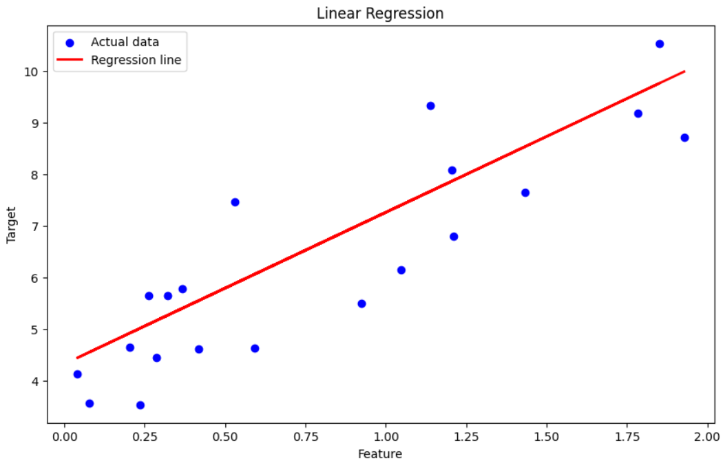
Sample Code Example

Linear Regression with Python - Predicting a Target Variable

        
            import numpy as np
            import matplotlib.pyplot as plt
            from sklearn.linear_model import LinearRegression
            from sklearn.model_selection import train_test_split
            from sklearn.metrics import mean_squared_error
            
            # Generate some synthetic data
            np.random.seed(0)
            X = 2 * np.random.rand(100, 1)  # Features
            y = 4 + 3 * X + np.random.randn(100, 1)  # Target
            
            # Split the data into training and testing sets
            X_train, X_test, y_train, y_test = train_test_split(X, y, test_size=0.2, random_state=0)
            
            # Create and train the model
            model = LinearRegression()
            model.fit(X_train, y_train)
            
            # Make predictions
            y_pred = model.predict(X_test)
            
            # Calculate the mean squared error
            mse = mean_squared_error(y_test, y_pred)
            print(f"Mean Squared Error: {mse}")
            
            # Plotting
            plt.figure(figsize=(10, 6))
            
            # Scatter plot of the test data
            plt.scatter(X_test, y_test, color='blue', label='Actual data')
            
            # Line plot of the predictions
            plt.plot(X_test, y_pred, color='red', linewidth=2, label='Regression line')
            
            plt.xlabel('Feature')
            plt.ylabel('Target')
            plt.title('Linear Regression')
            plt.legend()
            
            plt.show()
            
        
        Output:

AI-AlgoHub